This essay is based on Chapter 4 of Deep Learning for Coders with Fastai and PyTorch and the Practical Deep Learning for Coders course.
The explanations blend the book's material with my own understanding. The code is reorganized from my personal notebook into clear phases, with help from Claude AI, so it's easier to follow than the original exploratory version.
The best way to understand how a neural network actually learns is to build one without any shortcuts. No magic .fit() calls, no pretrained weights, just math, pixels, and gradients.
This article walks through building a digit classifier on the MNIST dataset, in five stages. Each stage makes the code more powerful and less manual. By the end, a single call classifies all 10 handwritten digits at 99% accuracy.
The Dataset
MNIST is a collection of 70,000 handwritten digit images, each 28×28 pixels in greyscale. We start with a simpler version: only 3s and 7s.
from fastai.vision.all import *
from fastbook import *

path = untar_data(URLs.MNIST_SAMPLE)
Path.BASE_PATH = path
path.ls()
[Path('labels.csv'), Path('train'), Path('valid')]
untar_data downloads and extracts the dataset to ~/.fastai/data/, caching it so it won't re-download on the next run. The folder has two splits, train for learning, valid for measuring how well we learned.
threes = (path/'train'/'3').ls().sorted()
sevens = (path/'train'/'7').ls().sorted()
len(threes), len(sevens)
(6131, 6265)
Each entry is a file path to a PNG image. Opening one:
img3 = Image.open(threes[1])
img3
It's just an image. But a computer sees it as a grid of numbers:
tensor(img3)tensor([[ 0, 0, 0, 0, 0, 0, 0, 0, 0, 0, 0, 0, 0, 0, 0, 0, 0, 0, 0, 0, 0, 0, 0, 0, 0, 0, 0, 0],
[ 0, 0, 0, 0, 0, 0, 0, 0, 0, 0, 0, 0, 0, 0, 0, 0, 0, 0, 0, 0, 0, 0, 0, 0, 0, 0, 0, 0],
[ 0, 0, 0, 0, 0, 0, 0, 0, 0, 0, 0, 0, 0, 0, 0, 0, 0, 0, 0, 0, 0, 0, 0, 0, 0, 0, 0, 0],
[ 0, 0, 0, 0, 0, 0, 0, 0, 0, 0, 0, 0, 0, 0, 0, 0, 0, 0, 0, 0, 0, 0, 0, 0, 0, 0, 0, 0],
[ 0, 0, 0, 0, 0, 0, 0, 0, 0, 0, 0, 0, 0, 0, 0, 0, 0, 0, 0, 0, 0, 0, 0, 0, 0, 0, 0, 0],
[ 0, 0, 0, 0, 0, 0, 0, 0, 0, 29, 150, 195, 254, 255, 254, 176, 193, 150, 96, 0, 0, 0, 0, 0, 0, 0, 0, 0],
[ 0, 0, 0, 0, 0, 0, 0, 48, 166, 224, 253, 253, 234, 196, 253, 253, 253, 253, 233, 0, 0, 0, 0, 0, 0, 0, 0, 0],
[ 0, 0, 0, 0, 0, 93, 244, 249, 253, 187, 46, 10, 8, 4, 10, 194, 253, 253, 233, 0, 0, 0, 0, 0, 0, 0, 0, 0],
[ 0, 0, 0, 0, 0, 107, 253, 253, 230, 48, 0, 0, 0, 0, 0, 192, 253, 253, 156, 0, 0, 0, 0, 0, 0, 0, 0, 0],
[ 0, 0, 0, 0, 0, 3, 20, 20, 15, 0, 0, 0, 0, 0, 43, 224, 253, 245, 74, 0, 0, 0, 0, 0, 0, 0, 0, 0],
[ 0, 0, 0, 0, 0, 0, 0, 0, 0, 0, 0, 0, 0, 0, 249, 253, 245, 126, 0, 0, 0, 0, 0, 0, 0, 0, 0, 0],
[ 0, 0, 0, 0, 0, 0, 0, 0, 0, 0, 0, 14, 101, 223, 253, 248, 124, 0, 0, 0, 0, 0, 0, 0, 0, 0, 0, 0],
[ 0, 0, 0, 0, 0, 0, 0, 0, 0, 11, 166, 239, 253, 253, 253, 187, 30, 0, 0, 0, 0, 0, 0, 0, 0, 0, 0, 0],
[ 0, 0, 0, 0, 0, 0, 0, 0, 0, 16, 248, 250, 253, 253, 253, 253, 232, 213, 111, 2, 0, 0, 0, 0, 0, 0, 0, 0],
[ 0, 0, 0, 0, 0, 0, 0, 0, 0, 0, 0, 43, 98, 98, 208, 253, 253, 253, 253, 187, 22, 0, 0, 0, 0, 0, 0, 0],
[ 0, 0, 0, 0, 0, 0, 0, 0, 0, 0, 0, 0, 0, 0, 9, 51, 119, 253, 253, 253, 76, 0, 0, 0, 0, 0, 0, 0],
[ 0, 0, 0, 0, 0, 0, 0, 0, 0, 0, 0, 0, 0, 0, 0, 0, 1, 183, 253, 253, 139, 0, 0, 0, 0, 0, 0, 0],
[ 0, 0, 0, 0, 0, 0, 0, 0, 0, 0, 0, 0, 0, 0, 0, 0, 0, 182, 253, 253, 104, 0, 0, 0, 0, 0, 0, 0],
[ 0, 0, 0, 0, 0, 0, 0, 0, 0, 0, 0, 0, 0, 0, 0, 0, 85, 249, 253, 253, 36, 0, 0, 0, 0, 0, 0, 0],
[ 0, 0, 0, 0, 0, 0, 0, 0, 0, 0, 0, 0, 0, 0, 0, 60, 214, 253, 253, 173, 11, 0, 0, 0, 0, 0, 0, 0],
[ 0, 0, 0, 0, 0, 0, 0, 0, 0, 0, 0, 0, 0, 0, 98, 247, 253, 253, 226, 9, 0, 0, 0, 0, 0, 0, 0, 0],
[ 0, 0, 0, 0, 0, 0, 0, 0, 0, 0, 0, 0, 42, 150, 252, 253, 253, 233, 53, 0, 0, 0, 0, 0, 0, 0, 0, 0],
[ 0, 0, 0, 0, 0, 0, 42, 115, 42, 60, 115, 159, 240, 253, 253, 250, 175, 25, 0, 0, 0, 0, 0, 0, 0, 0, 0, 0],
[ 0, 0, 0, 0, 0, 0, 187, 253, 253, 253, 253, 253, 253, 253, 197, 86, 0, 0, 0, 0, 0, 0, 0, 0, 0, 0, 0, 0],
[ 0, 0, 0, 0, 0, 0, 103, 253, 253, 253, 253, 253, 232, 67, 1, 0, 0, 0, 0, 0, 0, 0, 0, 0, 0, 0, 0, 0],
[ 0, 0, 0, 0, 0, 0, 0, 0, 0, 0, 0, 0, 0, 0, 0, 0, 0, 0, 0, 0, 0, 0, 0, 0, 0, 0, 0, 0],
[ 0, 0, 0, 0, 0, 0, 0, 0, 0, 0, 0, 0, 0, 0, 0, 0, 0, 0, 0, 0, 0, 0, 0, 0, 0, 0, 0, 0],
[ 0, 0, 0, 0, 0, 0, 0, 0, 0, 0, 0, 0, 0, 0, 0, 0, 0, 0, 0, 0, 0, 0, 0, 0, 0, 0, 0, 0]], dtype=torch.uint8)
Values range from 0 (black) to 255 (white). We load all images, stack them into a single block, and normalize values to [0.0, 1.0]:
three_tensors = [tensor(Image.open(o)) for o in threes]
stacked_threes = torch.stack(three_tensors).float() / 255
stacked_threes.shape
torch.Size([6131, 28, 28])
A 3D block: 6131 images × 28 rows × 28 columns. We then flatten each image into a single row of 784 numbers:
train_x = torch.cat([
    stacked_threes.view(-1, 28*28),
    stacked_sevens.view(-1, 28*28)
])
train_y = tensor([1]*len(threes) + [0]*len(sevens)).unsqueeze(1)
train_x.shape, train_y.shape
(torch.Size([12396, 784]), torch.Size([12396, 1]))
train_x is our input matrix, 12,396 images, each as 784 pixel values. train_y is our labels, 1 for threes, 0 for sevens.
We do the same for the validation set, then wrap everything in PyTorch DataLoaders that handle batching automatically:
dset = list(zip(train_x, train_y))
valid_dset = list(zip(valid_x, valid_y))

dl = DataLoader(dset, batch_size=256, shuffle=True)
valid_dl = DataLoader(valid_dset, batch_size=256, shuffle=False)
Phase 1 - The Bare Mechanics
Before using any library tools, we implement every piece by hand: weights, loss, and the gradient update loop.
Weights and a Linear Function
def init_params(size, std=1.0):
    return (torch.randn(size) * std).requires_grad_()

weights = init_params((28*28, 1))
bias    = init_params(1)

def linear1(xbatch):
    return xbatch @ weights + bias
weights holds one number per pixel, how much each pixel should matter. bias is a constant offset. @ is matrix multiplication: for a batch of images [256, 784] times weights [784, 1], we get [256, 1], one raw score per image.
.requires_grad_() tells PyTorch to track every operation on this tensor so it can compute gradients later.
Loss Function
Raw model scores can be any number. We need them as probabilities between 0 and 1 first, that's what sigmoid does:
plot_function(torch.sigmoid, title='Sigmoid', min=-10, max=10)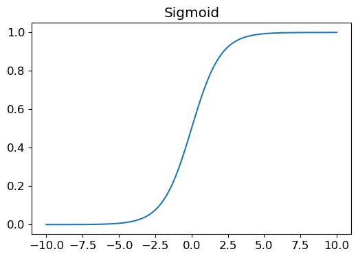
Then our loss penalizes wrong predictions:
def mnist_loss(predictions, targets):
    predictions = predictions.sigmoid()
    return torch.where(targets == 1, 1 - predictions, predictions).mean()
If the target is 1 (a three), we want the prediction close to 1, so the loss is 1 - prediction. If the target is 0 (a seven), we want the prediction close to 0, so the loss is the prediction itself. The .mean() gives us one number to optimize.
Gradients and the Update Loop
def calc_grad(xb, yb, model):
    preds = model(xb)
    loss  = mnist_loss(preds, yb)
    loss.backward()          # computes gradient of loss w.r.t. all parameters
loss.backward() uses the chain rule to compute how much each weight contributed to the error. It accumulates into .grad, so we zero it out after every update:
def train_epoch(model, lr, params):
    for xb, yb in dl:
        calc_grad(xb, yb, model)
        for p in params:
            p.data -= p.grad * lr    # nudge weights in the direction that reduces loss
            p.grad.zero_()
def validate_epoch(model):
accs = [batch_accuracy(model(xb), yb) for xb, yb in valid_dl]
return round(torch.stack(accs).mean().item(), 4)Training for 20 epochs:
lr = 1.
params = weights, bias
for i in range(20):
    train_epoch(linear1, lr, params)
    print(validate_epoch(linear1), end=" ")
0.8504 0.9007 0.9291 0.9388 0.9442 0.9525 0.9544 0.9588
0.9613 0.9623 0.9623 0.9632 0.9637 0.9647 0.9662 0.9667
0.9671 0.9671 0.9676 0.9681
From 54% (My first attempt on this notebook had the result starting at 0.54) to 96.8%, just from adjusting numbers based on errors. That's gradient descent.
Phase 2 - Cleaning Up with PyTorch
Manually managing weights and the update loop works, but PyTorch has built-in tools for this.
nn.Linear replaces our init_params + linear1 in one class. It also initializes weights smarter than random:
linear_model = nn.Linear(28*28, 1)We write a minimal optimizer class that formalizes our manual update loop. Notice *args and **kwargs in the methods, these absorb any extra arguments fastai might pass internally, so the method doesn't crash:
class BasicOptim:
    def __init__(self, params, lr):
        self.params, self.lr = list(params), lr

    def step(self, *args, **kwargs):
        for p in self.params:
            p.data -= p.grad.data * self.lr

    def zero_grad(self, *args, **kwargs):
        for p in self.params:
            p.grad = None
Then fastai's SGD replaces our BasicOptim, and Learner wraps the entire training loop:
dls   = DataLoaders(dl, valid_dl)
learn = Learner(dls, nn.Linear(28*28, 1), opt_func=SGD,
                loss_func=mnist_loss, metrics=batch_accuracy)
learn.fit(10, lr=1.)
epoch train_loss valid_loss batch_accuracy time
0 0.636894 0.503732 0.495584 00:00
1 0.630930 0.489802 0.495584 00:00
2 0.255438 0.315218 0.680569 00:00
3 0.108589 0.146847 0.869480 00:00
...
9 0.017803 0.040536 0.966143 00:00
Same math as before, now with less manual code.
Phase 3 - Adding Nonlinearity (This Is What Makes It a Neural Network)
A chain of linear layers always collapses into a single linear layer, no matter how deep you go. To learn complex patterns, we need a nonlinearity between layers.
The simplest one is ReLU: replace every negative number with zero.
plot_function(F.relu)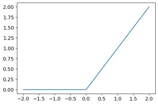
This tiny function is why deep learning works. Two linear layers with a ReLU between them can approximate any function, given enough hidden units.
simple_nnet = nn.Sequential(
    nn.Linear(28*28, 32),   # 784 pixels → 32 learned features
    nn.ReLU(),
    nn.Linear(32, 1)        # 32 features → 1 prediction
)
nn.Sequential runs each layer in order, passing the output of one as input to the next. The 32 in the middle is the number of hidden units, how many intermediate patterns the network can learn.
learn = Learner(dls, simple_nnet, opt_func=SGD,
                loss_func=mnist_loss, metrics=batch_accuracy)
learn.fit(40, 0.1)
epoch train_loss valid_loss batch_accuracy time
0 0.313917 0.406301 0.505397 00:00
1 0.145470 0.225546 0.809617 00:00
...
39 0.014229 0.020623 0.982336 00:00
Accuracy over training:
plt.plot(L(learn.recorder.values).itemgot(2))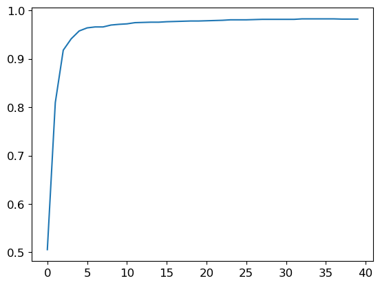
98.2%, better than the linear model, and it got there faster per epoch.
Phase 4 - All 10 Digits with ResNet18
Binary classification (3 vs 7) was a warm-up. The full problem is classifying all 10 handwritten digits.
Three things change from the binary setup:
- More classes: the output layer needs 10 neurons, one per digit
- Loss function:
F.cross_entropyreplaces our custommnist_loss, and handles multi-class naturally - Architecture: a deeper model can learn richer features
Instead of building everything manually again, we use fastai's high-level API, which is exactly the payoff of understanding all the phases above:
dls = ImageDataLoaders.from_folder(untar_data(URLs.MNIST))

learn = vision_learner(
    dls, resnet18,
    pretrained=False,
    loss_func=F.cross_entropy,
    metrics=accuracy
)
learn.fit_one_cycle(1, 0.1)
epoch train_loss valid_loss accuracy time
0 0.065941 0.018110 0.994603 00:07
99.5% accuracy. One epoch. Seven seconds.
fit_one_cycle uses a learning rate schedule that starts low, ramps up, then comes back down, it trains significantly faster than a flat learning rate.
ResNet18 is an 18-layer convolutional network with skip connections that let gradients flow through deep layers without vanishing. It's the same architecture used in real computer vision pipelines, and it works here with zero pretrained weights, purely from learning on MNIST.
What This All Means
Here's the full arc:
| Phase | Approach | Accuracy |
|---|---|---|
| 1 | Manual weights + gradient loop | 96.8% |
| 2 | nn.Linear + custom optimizer | 97.8% |
| 3 | 2-layer network + ReLU | 98.2% |
| 4 | ResNet18, all 10 digits | 99.5% |
Each step removed manual code and added expressive power. The math never changed , the abstractions just got better at expressing it.
Understanding what loss.backward() actually does, why you zero gradients, and why nonlinearity matters is what lets you reason about why a model isn't learning, instead of just trying things and hoping.
Honestly, I originally wrote this for myself as a reference, but I thought it might be helpful to share it with others too. So here's something useful for both of us:
Neural Network Concepts (Quick Reference)
Linear Model Limits
Linear = straight lines only. Can't learn curved boundaries. Need ReLU/hidden layers for non-linearity.
Gradient
Slope pointing downhill. Tells you which direction to move weights to reduce loss. Calculated via backprop.
Batches
Average 256 images' signal instead of 1 (less noisy). Also: GPU processes batch in ~same time as 1 image.
ReLU
max(0, x) -> kills negatives. Without it, stacking layers = no extra power. ReLU adds non-linearity.
Loss Function
Distance from truth. Lower = better predictions. Model learns by minimizing it.
Training vs Validation Loss
Training = data model saw. Validation = data it didn't. If validation >> training = overfitting (memorized).
Batching Cheat Sheet
from torch.utils.data import TensorDataset, DataLoader

# Pair data
dset = TensorDataset(train_x, train_y)

# Create batches (start with 128)
train_dl = DataLoader(dset, batch_size=128, shuffle=True)

# Use in loop
for xb, yb in train_dl:
    # train on batch
Batch size: 64-256 is safe. Increase if slow, decrease if unstable.
Training Loop Pattern
- Forward:
preds = model(batch_x) - Loss:
loss = loss_func(preds, batch_y) - Backward:
loss.backward() - Update:
opt.step()→opt.zero_grad() - Repeat for all batches (= 1 epoch)